Human input wait is the gap, within one session, from the previous event of any type to each user_message. It is provider-agnostic (the shared timing.human_waits_from_event_pairs): the gap spans non-output events such as Codex usage_report, and every user message counts, not only turn-triggering ones. It is computed by a stateful single-pass walk over agent steps in ingestion order (round_pk == file order), keeping last_event_at_by_session: {session_id -> datetime}. For each step, in event time order:

1. For each user_message event with a recorded previous-event timestamp prev for the session, the wait is (user_ts − prev).total_seconds(); when strictly positive it is appended to the "all" list and to that step’s provider bucket.
2. prev advances to every event’s timestamp as the walk passes it (so consecutive user→user gaps count too), carrying across rounds via last_event_at_by_session.

This is a trace-level estimate, not a serving-engine timer; it reflects only recorded events. The wait spans the human think/read time between requests and excludes the model’s own generation.

Note (definition change). Earlier this metric used previous model output → response-triggering user message, which dropped non-trigger messages and Codex’s post-output usage_report tail — undercounting Codex idle (it surfaced elsewhere as an unattributed “Other” residual). The current provider-agnostic definition captures all human idle (Claude ≈ 90%, Codex ≈ 94% of session wall-clock).

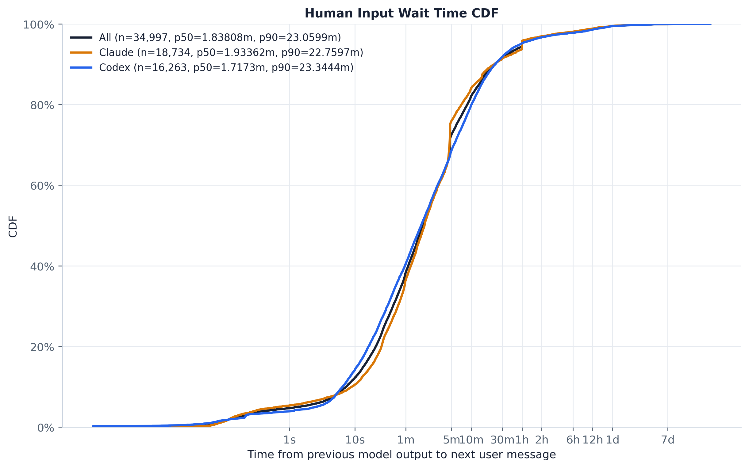
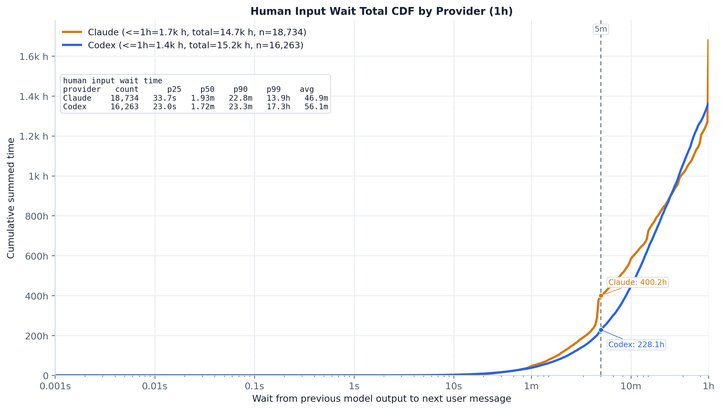
The experiment renders the wait distribution three ways, with the x-axis on a log duration scale and the count/total panels capped at 1h (a 5-minute reference line marks a plausible cache-eviction horizon):

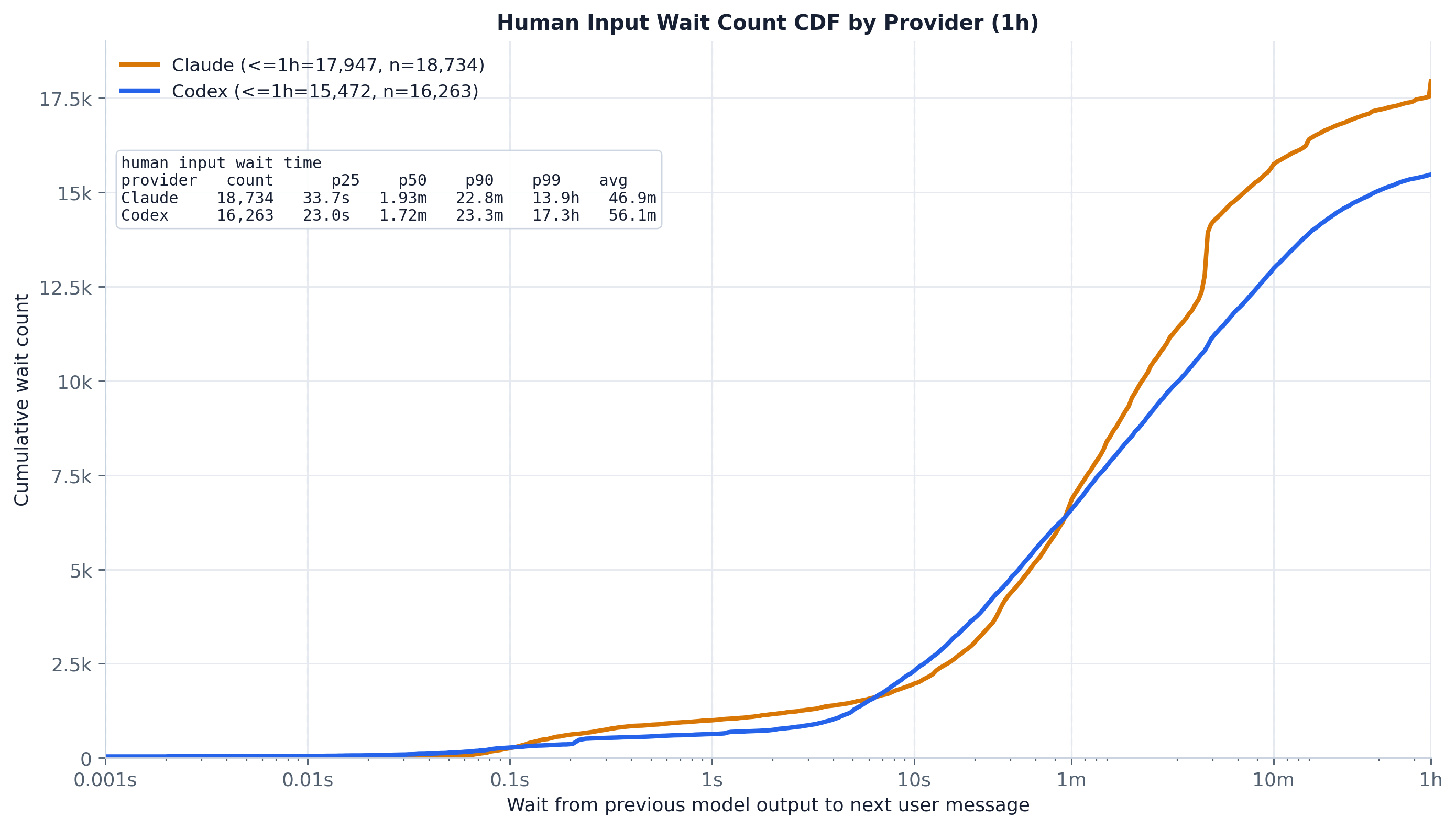
• a single-axis wait CDF overlaying all and each provider;
• a per-provider count CDF — fraction of waits ≤ T;
• a per-provider total CDF — share of summed idle time from waits ≤ T.

Method and assumptions:

• Exact, not sampled. Every positive wait contributes one value to its provider’s list (and to all); the CDFs, percentiles, and summed-time bins run over the full set. The old loader already kept every wait here — there was never a reservoir cap on this metric — so the migration is value-for-value identical.
• File-order state. The walk is over round_pk (ingestion ordinal == file order), reproducing the line-order tie-break the old single-pass JSONL loader relied on for its session state.
• Provider grouping mirrors the old loader’s str(provider) or "<unknown-provider>" fallback, so a missing/empty provider falls into <unknown-provider>.
• Engine-independent timestamps. Timestamps are read from the DB as integer epoch-microseconds (CAST(epoch_us(timestamp) AS BIGINT)) and rebuilt to naive datetimes in Python, never fetched as a raw TIMESTAMP (native duckdb marshals that to a datetime, duckdb-wasm to a string). A difference between two same-timezone datetimes equals the naive-microsecond difference exactly, so the waits match the pre-DuckDB result bit-for-bit.

plot.py is a query→shape→plot pipeline over the shared trace DuckDB:

• load_human_input_wait_seconds_by_provider(con) — the only data-loading code. It pulls per-step timing_events (event_type + epoch-microsecond timestamp, in round_pk ingest order) and the per-step (session_id, provider) from rounds, then runs the stateful walk above, returning {"all": [...], provider: [...]}. The full per-provider lists are returned, no sampling.
• timing.human_waits_from_event_pairs(...) — the shared, provider-agnostic core (imported from artifacts/utils/timing.py): given a session’s (event_type, timestamp) pairs and the carried previous-event time, it walks them in time order and returns the positive previous-event→user_message waits. The same helper backs the row-dict consumers (trace_loader, overview_summary), so every path computes identical waits.
• _epoch_us_to_datetime(...) — rebuilds a naive datetime from epoch-microseconds.
• ordered_human_wait_items / human_wait_summary_row / plot_human_input_wait_cdf / write_human_input_wait_summary — shape the overlay CDF and the summary CSV (unchanged from the pre-migration script).
• The count/total figures and their CSVs are produced by the shared cdf.py helpers (plot_count_cdf_by_provider / plot_cumulative_duration_cdf_by_provider and their write_* counterparts) — matplotlib/CSV behavior unchanged.
• main() — wires the standard trace_db CLI (--db | -i/--input | -o/--output-dir) and embeds the self-contained PNG sidecar.

The data layer (parsing, surrogate keys, schema) lives in artifacts/utils/trace_db.py; see artifacts/utils/DB_SCHEMA.md.

# default merged trace, output next to this README
uv run python artifacts/human_in_the_loop/human_input_wait/plot.py

# a specific trace (materialized to a temp DuckDB cache on first use)
uv run python artifacts/human_in_the_loop/human_input_wait/plot.py -i trace/sample.jsonl

# a prebuilt DB (run_all.py's build-db step passes this), into a chosen dir
uv run python artifacts/human_in_the_loop/human_input_wait/plot.py --db "$TMPDIR/trace.duckdb" -o "$TMPDIR/out"

• human_input_wait_cdf.png — single-axis wait CDF overlaying all and each provider, with n/p50/p90 in the legend.
• human_input_wait_count_cdf_by_provider.png / .csv — per-provider count CDF over the wait threshold (waits ≤ T), with per-bin and cumulative counts/shares.
• human_input_wait_total_cdf_by_provider.png / .csv — per-provider summed-idle-time CDF, with per-bin seconds/hours and cumulative time shares.
• human_input_wait_summary.csv — per-group (all + providers) count, mean, p50/p90/p95/p99, and max in seconds.

Each PNG embeds this README, the CSVs above, and the plotting code (plot.py + shared artifacts/utils/ modules) as compressed text chunks. Unpack with uv run python artifacts/utils/png_sidecar.py extract <png>.