
How many tokens does the model generate per agent step, and how does that distribution differ by provider / model?
How many tokens does the model generate per agent step, and how does that distribution differ by provider / model?
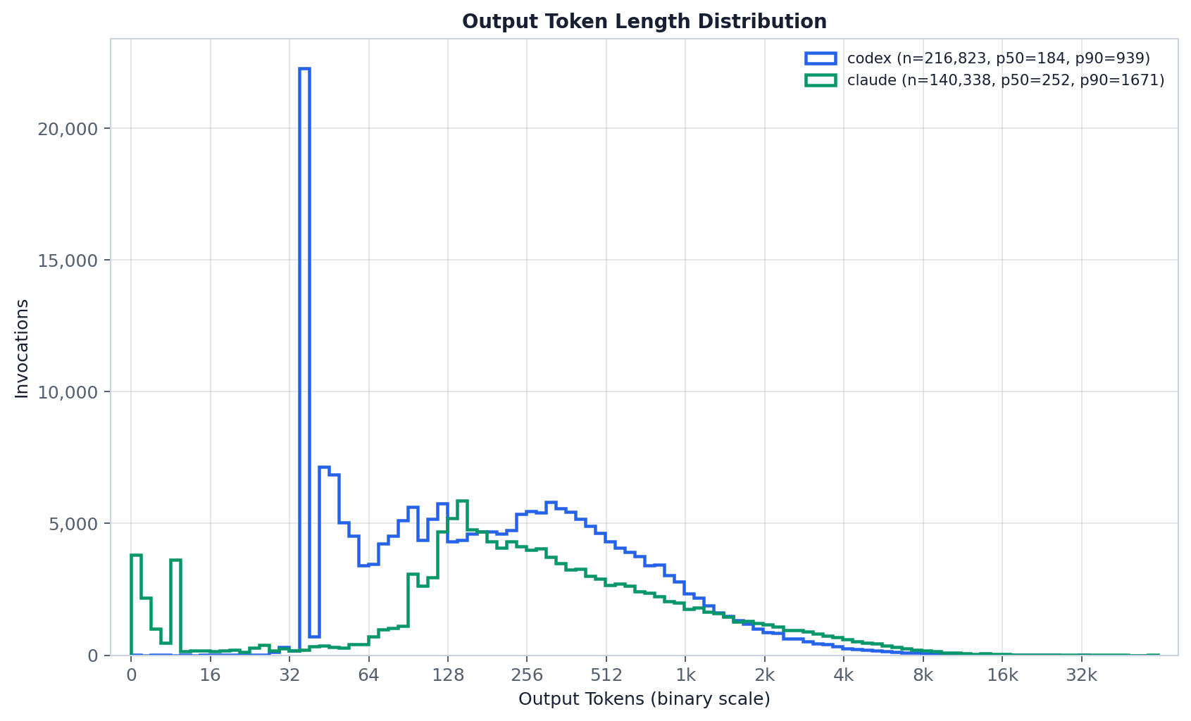
The full per-step output distribution (the paper’s fig:output_tokens): both providers pile up in
the low hundreds of tokens — median 354 for Claude, 188 for Codex — and the curve is strongly
right-skewed, with only a thin tail of long generations reaching the per-group max. Outputs
this short are the expected consequence of the tool loop: a full response is cut into 6.7 tool-call
steps, so most steps emit just the next call’s arguments rather than a long answer. Codex adds a
distinctive second feature — a pronounced spike of very short (~40-token) generations — driven by its
heavy use of write_stdin to wait on a running command or send Ctrl+C to interrupt one. Read the
curves side by side rather than overlaying one number: Codex folds reasoning tokens into
output_tokens while Claude does not, so a heavier Codex tail can reflect reasoning rather than more
visible output, and the <unknown-*> buckets (if present) flag steps with missing provenance.
For every agent step the trace records output_tokens — the step’s generated-token count. This
experiment plots the distribution of that count, grouped by provider (or model, or
provider:model), on a base-2 log token axis, and writes per-group quantiles.
Method and assumptions:
output_tokens is non-null and >= 0 contributes one value to
its group (and to the synthetic all group). This follows the JSONL loader’s allow_zero numeric
rule — zero-output steps are kept, negatives (never observed) are dropped.output_tokens includes reasoning tokens; for Claude it
is the message-level output count. The distributions are therefore not strictly like-for-like
across providers — read each provider on its own terms.sampled column is therefore always False and sample_count equals the full
count. (On any trace below the 200k cap — e.g. trace/sample.jsonl — that path is exact.)group_key() "<unknown-provider>" /
"<unknown-model>" fallbacks via SQL COALESCE, so missing/empty provider or model values fall
into an explicit <unknown-*> bucket rather than being dropped.plot.py is a query→shape→plot pipeline over the shared trace DuckDB:
load_metric_by_group(con, *, column, group_by) — the only data-loading code. It pulls every
non-null, non-negative output_tokens value with its group label (one SQL GROUP BY-free scan)
and returns {group_label: MetricStats} plus an all group. No sampling.MetricStats — a thin wrapper over the group’s full np.ndarray of values, exposing exact
count / min / max / mean and percentiles(...) (NumPy linear interpolation).selected_groups(stats, max_groups) — the plotted groups: everything except all, biggest first,
capped at --max-groups.plot_output_tokens(...) — renders the stepped histogram on the shared binary token axis
(formatters.token_axis_*, style.*); matplotlib behavior unchanged from the pre-migration script.write_output_token_summary(...) — the per-group quantile CSV.main() — wires the standard trace_db CLI (--db | -i/--input | -o/--output-dir), plus
--group-by and --max-groups, and embeds the self-contained PNG sidecar.The data layer (parsing, surrogate keys, schema) lives in artifacts/utils/trace_db.py; see
artifacts/utils/DB_SCHEMA.md.
# against the shared DuckDB built by run_all (no per-script re-parse)
uv run python artifacts/llm_generation/output_tokens/plot.py --db "$TMPDIR/trace.duckdb"

# or straight from a JSONL trace (materialized to a temp cache on first use)
uv run python artifacts/llm_generation/output_tokens/plot.py -i trace/sample.jsonl

# group by model instead of provider, show more groups
uv run python artifacts/llm_generation/output_tokens/plot.py -i trace/sample.jsonl --group-by model --max-groups 12
output_tokens_distribution.png — per-group output-token histogram on a base-2 token axis; the
legend reports each group label.output_tokens_summary.csv — per-group quantiles: count, min, p50, p90, p95, p99, max, mean,
plus sample_count (= count) and sampled (always False, since the stats are exact).The PNG is self-contained: it embeds this README, output_tokens_summary.csv, and the plotting code
as compressed text chunks. Unpack with uv run python artifacts/utils/png_sidecar.py extract <png>.