SyFI Trace Atlas
Trace assistant
Reading the public SYFI pool
357,161 agent steps across Claude & Codex — public, shareable.
Answers run real DuckDB/Python in a sandbox · code is shown
All figures
Session
one continuous trace of work, often spanning multiple requests or problems.
Request
one user input through the agent's final response.
Agent step
one model call inside a request.
User-initiated step
an agent step started by user input.
Tool-triggered step
an agent step started by a tool result.
Overview

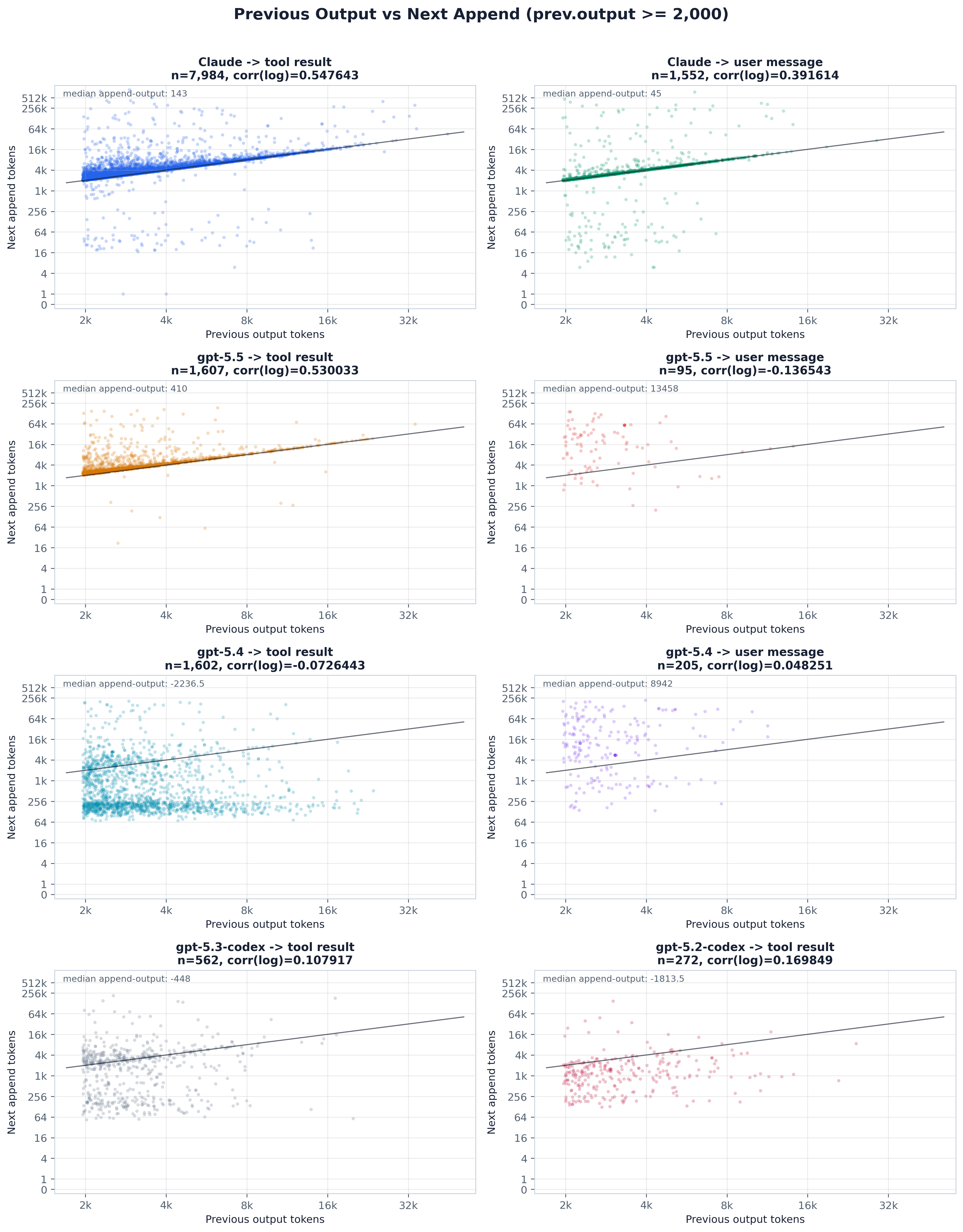
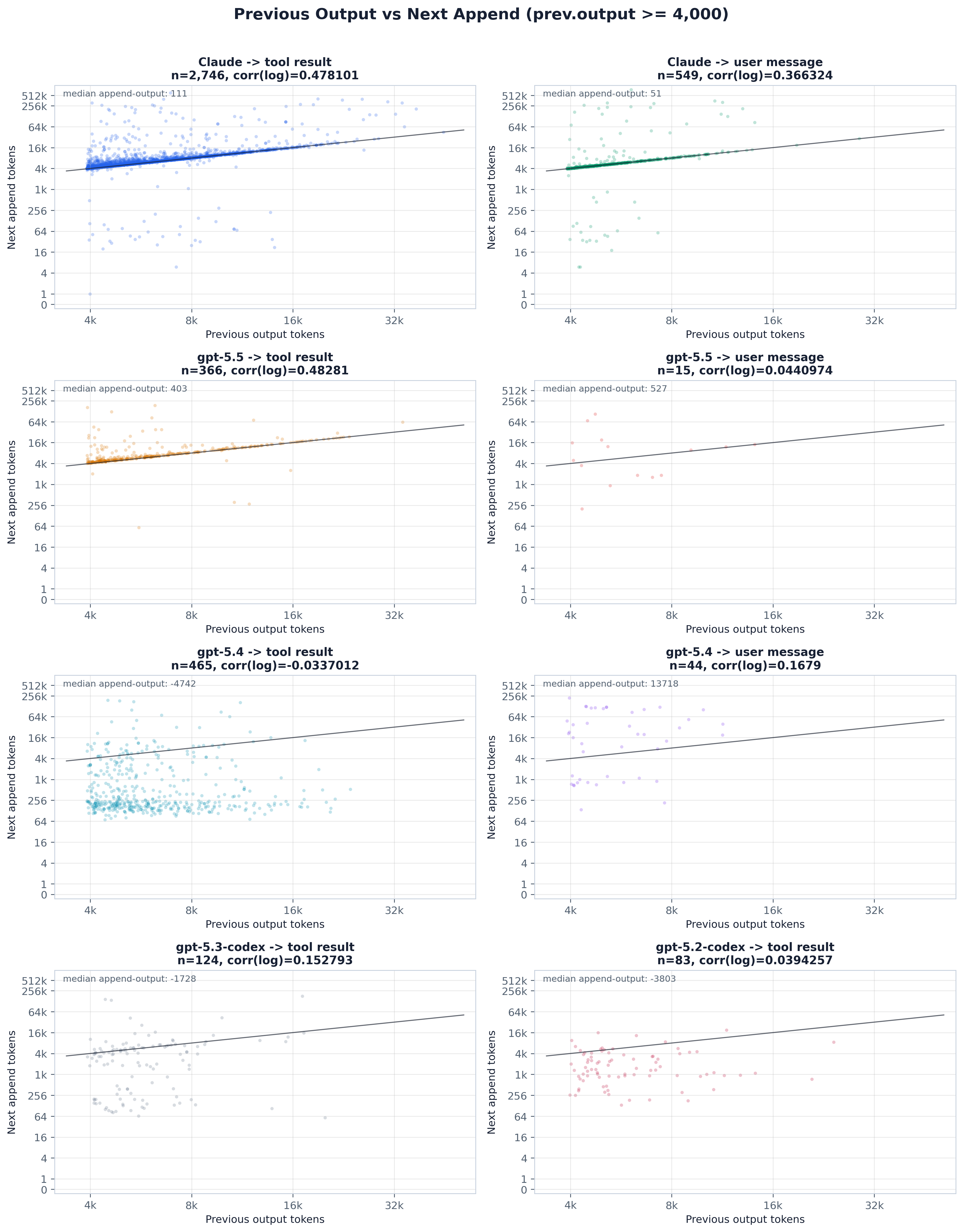
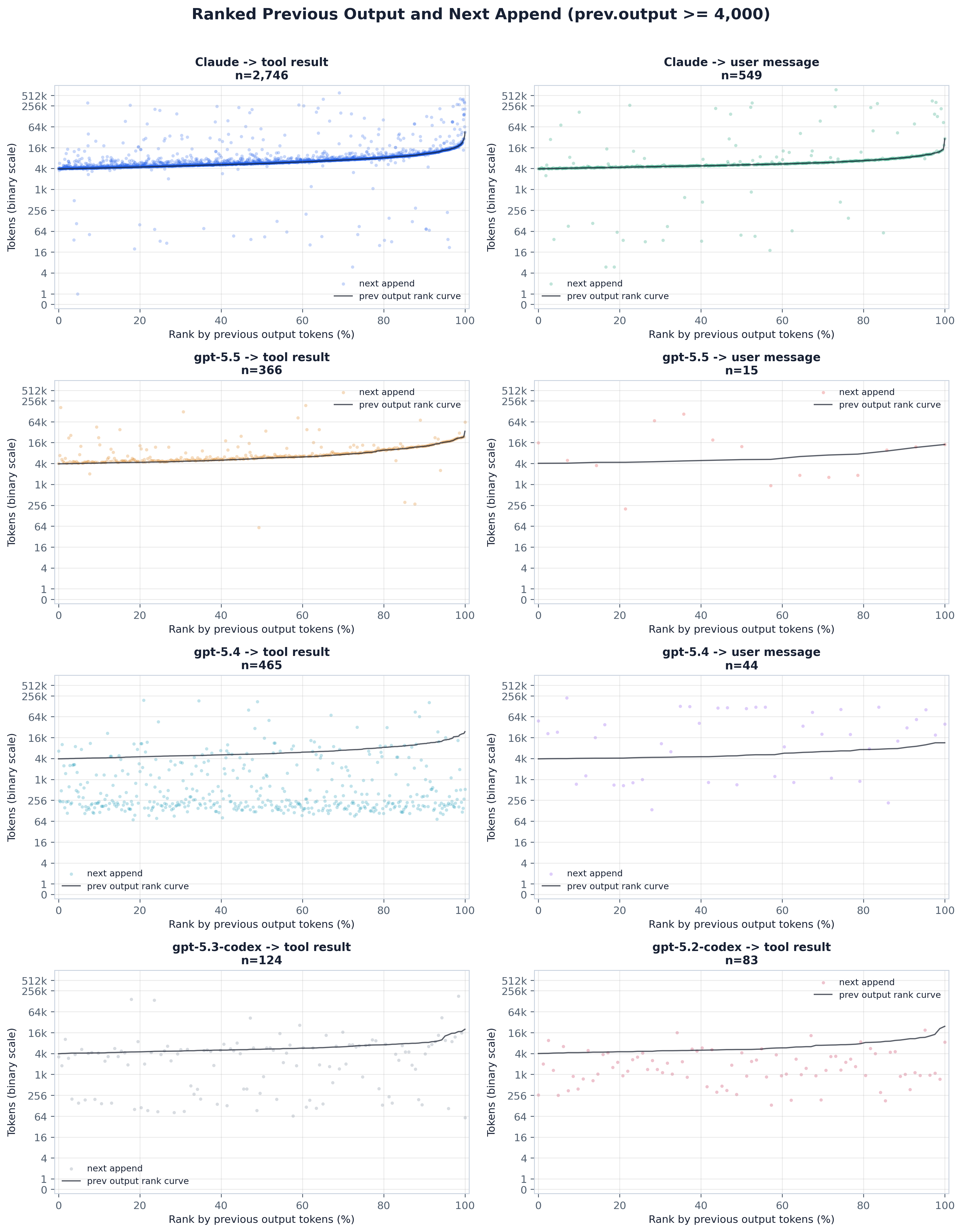
Does an agent step’s output token count predict the next step’s newly appended tokens (i.e. is the prior response what reappears as new append), and how does prior output relate to the next step’s cached-prefix gain — does the previous response land on the prefix side or the append side?

The previous assistant response is normally replayed into the next prompt. This experiment asks where it lands by comparing adjacent agent steps in the same session: prev.output_tokens against the 
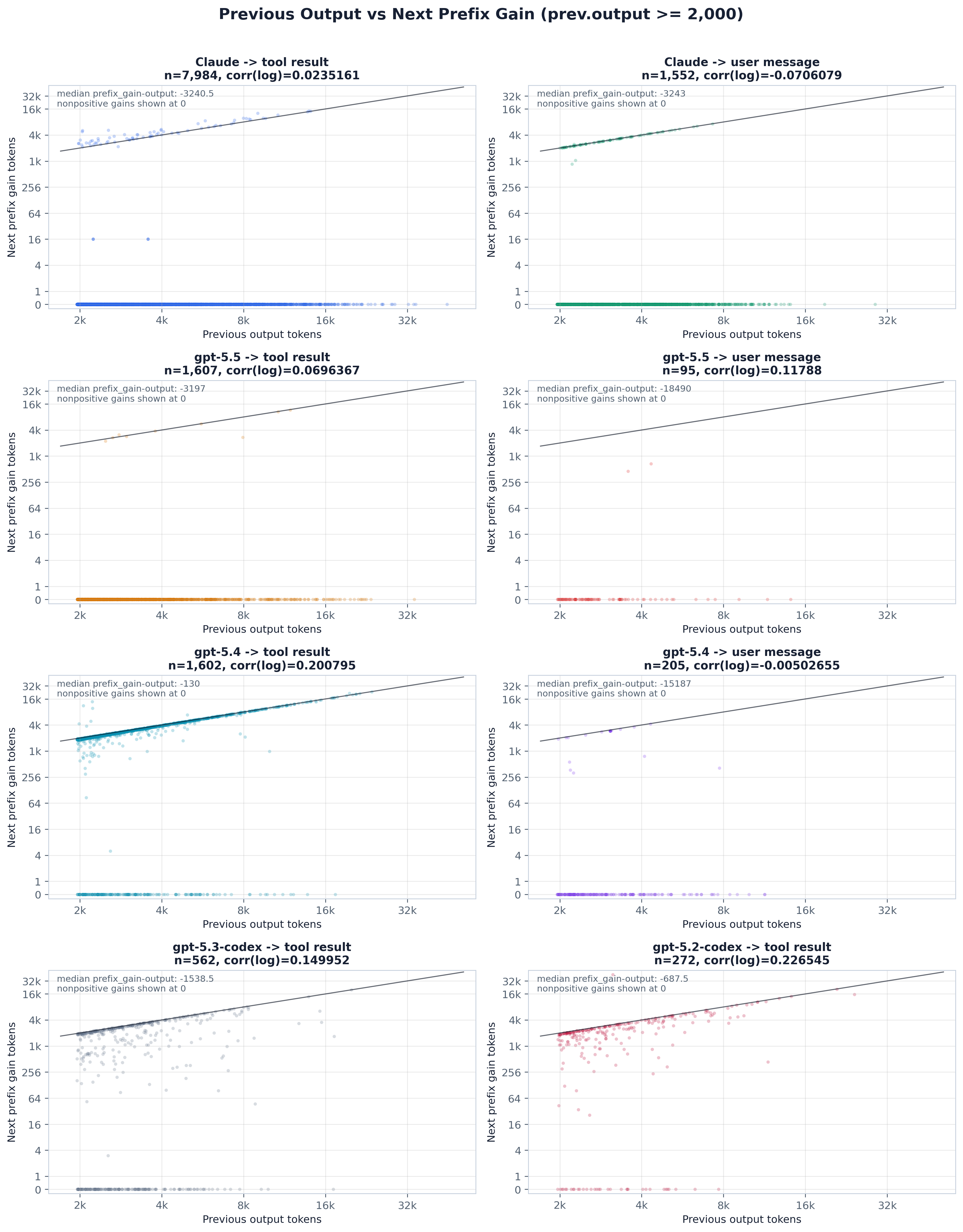
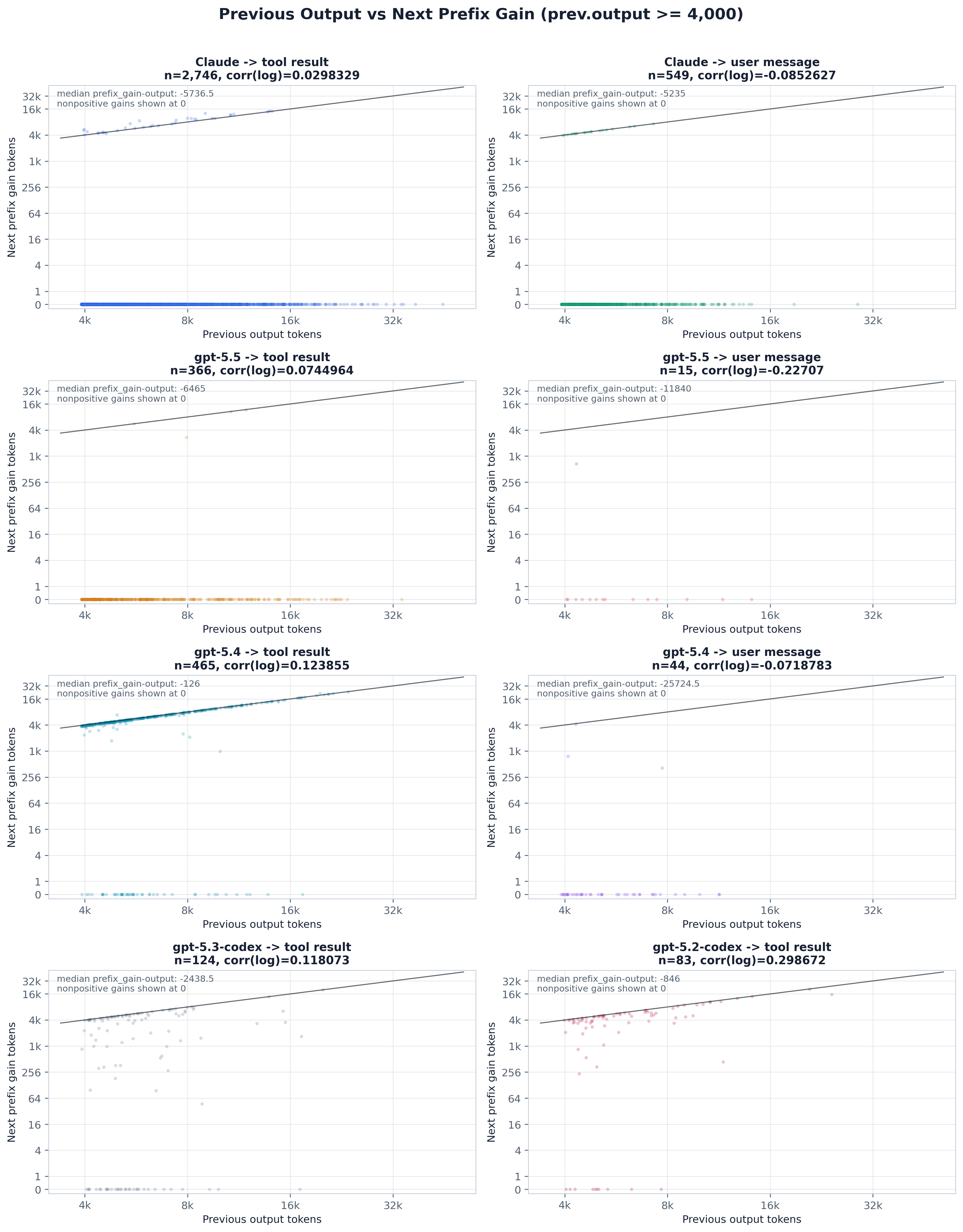
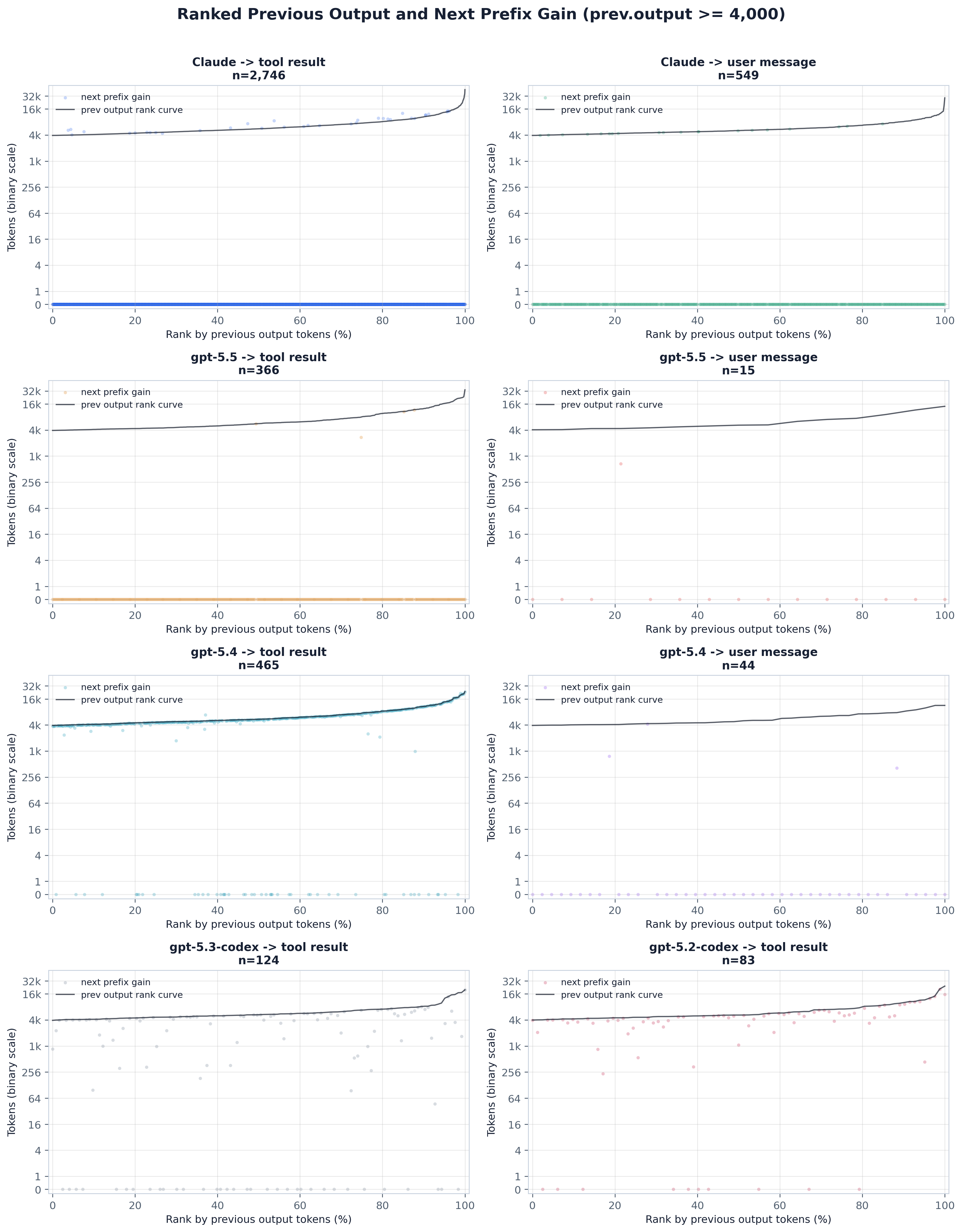
next step’s newly_append_tokens (the freshly charged slice) and against the next step’s prefix gain (current.prefix_tokens − previous.input_tokens_total). It tests the replay hypothesis from ../../../docs/prompt_cache_accounting.md: the prior response generally shows up in the next step’s append/cache-write.

Method and assumptions:

  • Adjacent agent steps within a session. Steps are grouped per (provider, session_id), sorted by (round_index, first-event timestamp), and each step is paired with the one immediately after it in that sorted order. (Unlike adjusted_prefix_append, pairs are adjacency-in-order, not a strict round_index step of 1.)
  • A timing gap gates each pair. The gap from the previous step’s last model-output event (reasoning/text/tool_call, falling back to its first observed timestamp) to the current step’s first observed timestamp must be ≥ 0 and ≤ --max-gap-seconds (default 240) — this drops cross-conversation or stale pairs. Pairs whose previous step has non-positive input_tokens_total or output_tokens are skipped.
  • Scenarios split pairs by provider/model and by how the next step started (tool_result vs user_message): Claude, gpt-5.5, gpt-5.4, gpt-5.3-codex, gpt-5.2-codex.
  • Assignment heuristic. Per pair, with a per-pair tolerance max(512, 0.10·prev_output): prefix_close (prefix gain ≈ prev output), prefix_rejects_output (prefix gain far below prev output), append_can_contain_output, and append_side_pair (= reject ∧ can-contain). The per-scenario prefix_close_pct / append_side_pair_pct drive a decision label (prefix_side / append_side / mixed / not_sure) and a decision_strength.
  • Output proxy. Output is taken as the step’s raw output_tokens. For Codex, output includes reasoning, so the visible-output proxy output_tokens − reasoning_output_tokens is reported as context in the method notes (the carried prev_reasoning is recorded per pair), but the plotted quantity is output_tokens.
  • Thresholds (--min-output-tokens, default 2000 4000) drop tiny-output noise; one full set of figures + summary is emitted per threshold N.
  • Stats are exact. Every percentile / correlation in the summary CSV is computed over all pairs in the scenario (legacy linear-interpolation percentile, (n−1)·q); nothing is sampled for the stats.
  • Adjacency ordering is file order. The pre-migration JSONL loader grouped rows per (provider, session_id) in first-appearance (file) order, then stably sorted each session by (round_index, first_timestamp) so ties kept file order. The shared DuckDB surrogate key ingest_seq (= round_pk) is that file order, so pulling ORDER BY ingest_seq and grouping in Python reproduces both the per-session row order and the session-visitation order byte-for-byte. This matters for the scatter: the per-scenario subsample’s stable sort by prev_output keeps the pair-append order on ties, and that append order is driven by the session-visitation order.
Figures 8
Previous output versus next append, min 2000 output tokens.
Fig. 1Previous output versus next append, min 2000 output tokens.

One scatter panel per scenario on base-2 log axes: x = previous step’s output tokens, y = next step’s newly appended tokens, with the y = prev.output diagonal and a per-panel corr(log) and median append − output.

  • Points hugging the diagonal are the replay signal — the previous response reappears nearly one-for-one in the next step’s append. Scenarios where the cloud sits on or above the line are append-side; clouds well below it mean the prior output did not land in append.
  • The threshold N (2000 vs 4000) trims small-output pairs; the larger threshold sharpens the high-output regime where replay is easiest to see.
  • The panel is a per-scenario subsample (up to --max-points-per-scenario), so it conveys joint structure, not exact density — read the summary CSV for the per-scenario percentages and decision.
Ranked previous output and next append, min 2000 output tokens.
Fig. 2Ranked previous output and next append, min 2000 output tokens.

The same data ranked: x = percentile rank by previous output, the black curve is the sorted prev-output sweep, scattered points are the next append at each rank. It separates “do append and output rise together” (curve and cloud track) from level-shift gaps, and is robust to the heavy-tailed token distribution that compresses the raw scatter.

Previous output versus next prefix gain, min 2000 output tokens.
Fig. 3Previous output versus next prefix gain, min 2000 output tokens.

x = previous output, y = next step’s prefix gain (current.prefix_tokens − previous.input_tokens_total, non-positive gains drawn at 0), with the y = prev.output diagonal and a median prefix_gain − output.

  • Points on the diagonal are the prefix side: the prior output was absorbed into the next step’s cached prefix rather than re-charged as append. A scenario that is on-diagonal here and below-diagonal in the append scatter is prefix_side in the CSV.
  • Gains pinned at 0 (or below the line) mean the prior output did not grow the cached prefix — the append side, or a cache miss.
Ranked previous output and prefix gain, min 2000 output tokens.
Fig. 4Ranked previous output and prefix gain, min 2000 output tokens.

The ranked counterpart for prefix gain: x = percentile rank by previous output, black curve = sorted prev-output sweep, scatter = next prefix gain at each rank. Reads like the append rank grid but for the cached-prefix side, making it easy to see at which output magnitudes the prior response starts landing on the prefix.

Previous output versus next append, min 4000 output tokens.
Fig. 5Previous output versus next append, min 4000 output tokens.

One scatter panel per scenario on base-2 log axes: x = previous step’s output tokens, y = next step’s newly appended tokens, with the y = prev.output diagonal and a per-panel corr(log) and median append − output.

  • Points hugging the diagonal are the replay signal — the previous response reappears nearly one-for-one in the next step’s append. Scenarios where the cloud sits on or above the line are append-side; clouds well below it mean the prior output did not land in append.
  • The threshold N (2000 vs 4000) trims small-output pairs; the larger threshold sharpens the high-output regime where replay is easiest to see.
  • The panel is a per-scenario subsample (up to --max-points-per-scenario), so it conveys joint structure, not exact density — read the summary CSV for the per-scenario percentages and decision.
Ranked previous output and next append, min 4000 output tokens.
Fig. 6Ranked previous output and next append, min 4000 output tokens.

The same data ranked: x = percentile rank by previous output, the black curve is the sorted prev-output sweep, scattered points are the next append at each rank. It separates “do append and output rise together” (curve and cloud track) from level-shift gaps, and is robust to the heavy-tailed token distribution that compresses the raw scatter.

Previous output versus next prefix gain, min 4000 output tokens.
Fig. 7Previous output versus next prefix gain, min 4000 output tokens.

x = previous output, y = next step’s prefix gain (current.prefix_tokens − previous.input_tokens_total, non-positive gains drawn at 0), with the y = prev.output diagonal and a median prefix_gain − output.

  • Points on the diagonal are the prefix side: the prior output was absorbed into the next step’s cached prefix rather than re-charged as append. A scenario that is on-diagonal here and below-diagonal in the append scatter is prefix_side in the CSV.
  • Gains pinned at 0 (or below the line) mean the prior output did not grow the cached prefix — the append side, or a cache miss.
Ranked previous output and prefix gain, min 4000 output tokens.
Fig. 8Ranked previous output and prefix gain, min 4000 output tokens.

The ranked counterpart for prefix gain: x = percentile rank by previous output, black curve = sorted prev-output sweep, scatter = next prefix gain at each rank. Reads like the append rank grid but for the cached-prefix side, making it easy to see at which output magnitudes the prior response starts landing on the prefix.

Reference

Code structure

plot.py is a query→shape→plot pipeline over the shared trace DuckDB:

  • load_pairs(con, *, max_gap_seconds) — pulls the step-level columns ORDER BY ingest_seq and the per-step timing events ORDER BY round_pk, event_index (timestamps as epoch_us integers, rebuilt to naive datetimes for native/wasm-identical marshalling), drops rows with a non-string provider/session_id, a non-integer round_index, or no observed timestamp (the old loader’s validity gate; in the pinned-schema DB these are the NULL rows), groups into rows_by_session preserving file order, stably sorts each session by (round_index, first_timestamp), then walks adjacent pairs applying the gap gate. Returns the list of Pairs.
  • first_timestamp(...) / last_model_output_timestamp(...) — first observed and last model-output timestamps of a step, over its timing events in event_index order, unchanged in semantics from pre-migration.
  • The assignment predicates (prefix_close, prefix_rejects_output, append_can_contain_output, append_side_pair, assignment_label) and scenario_groups() — unchanged.
  • plot_scatter_grid / plot_rank_grid / plot_prefix_gain_scatter_grid / plot_prefix_gain_rank_grid — the four figure families; sampled_pairs(...) is the per-scenario scatter decimation (deterministic rank-stratified np.linspace over a stable prev_output sort).
  • write_summary(...) — the per-scenario decision/quantile CSV, using the legacy percentile / fmt helpers so values match the pre-migration run exactly.
  • main() — wires the standard trace_db CLI (--db | -i/--input | -o/--output-dir), keeps the custom --max-gap-seconds / --min-output-tokens / --max-points-per-scenario flags, and embeds the self-contained PNG sidecar.

The data layer (parsing, surrogate keys, schema) lives in artifacts/utils/trace_db.py; see artifacts/utils/DB_SCHEMA.md.

Running it

# default merged trace, output next to this README
uv run python artifacts/llm_generation/output_append_assignment/plot.py

# a specific trace (materialized to a temp DuckDB cache on first use)
uv run python artifacts/llm_generation/output_append_assignment/plot.py -i trace/sample.jsonl

# a prebuilt DB (run_all.py's build-db step passes this), into a chosen dir
uv run python artifacts/llm_generation/output_append_assignment/plot.py --db /tmp/trace.duckdb -o /tmp/out

Useful flags: --max-gap-seconds (pair gap ceiling, default 240), --min-output-tokens (one figure set per threshold, default 2000 4000), --max-points-per-scenario (scatter/rank subsample per scenario, default 6000).

Outputs

Written to -o (default this folder), one set per --min-output-tokens threshold N:

  • output_vs_next_append_scatter_min{N}.png — prev-output vs next-append scatter grid.
  • ranked_output_vs_next_append_min{N}.png — ranked prev-output / next-append grid.
  • output_vs_prefix_gain_scatter_min{N}.png — prev-output vs next-prefix-gain scatter grid.
  • ranked_output_vs_prefix_gain_min{N}.png — ranked prev-output / next-prefix-gain grid.
  • output_append_assignment_summary_min{N}.csv — per-scenario count, decision, decision_strength, the log-output correlations, the prefix_close / prefix_reject / append_can_contain_output / append_side_pair / unassigned percentages, and the median / p10 / p90 token quantiles (over all pairs).

Each PNG is self-contained — it embeds this README, the summary CSVs, and the plotting code (plot.py + shared artifacts/utils/ modules). Unpack with python artifacts/utils/png_sidecar.py extract <png>.

SyFI Trace Atlas · experiment detail