SyFI Trace Atlas
Trace assistant
Reading the public SYFI pool
357,161 agent steps across Claude & Codex — public, shareable.
Answers run real DuckDB/Python in a sandbox · code is shown
All figures
Session
one continuous trace of work, often spanning multiple requests or problems.
Request
one user input through the agent's final response.
Agent step
one model call inside a request.
User-initiated step
an agent step started by user input.
Tool-triggered step
an agent step started by a tool result.
Overview

How long do tool calls take, per tool and per provider, and where does the long tail of tool latency live — for Claude Code vs Codex?

Every agent step carries a tools[] list of tool calls, each with a measured latency. This experiment 
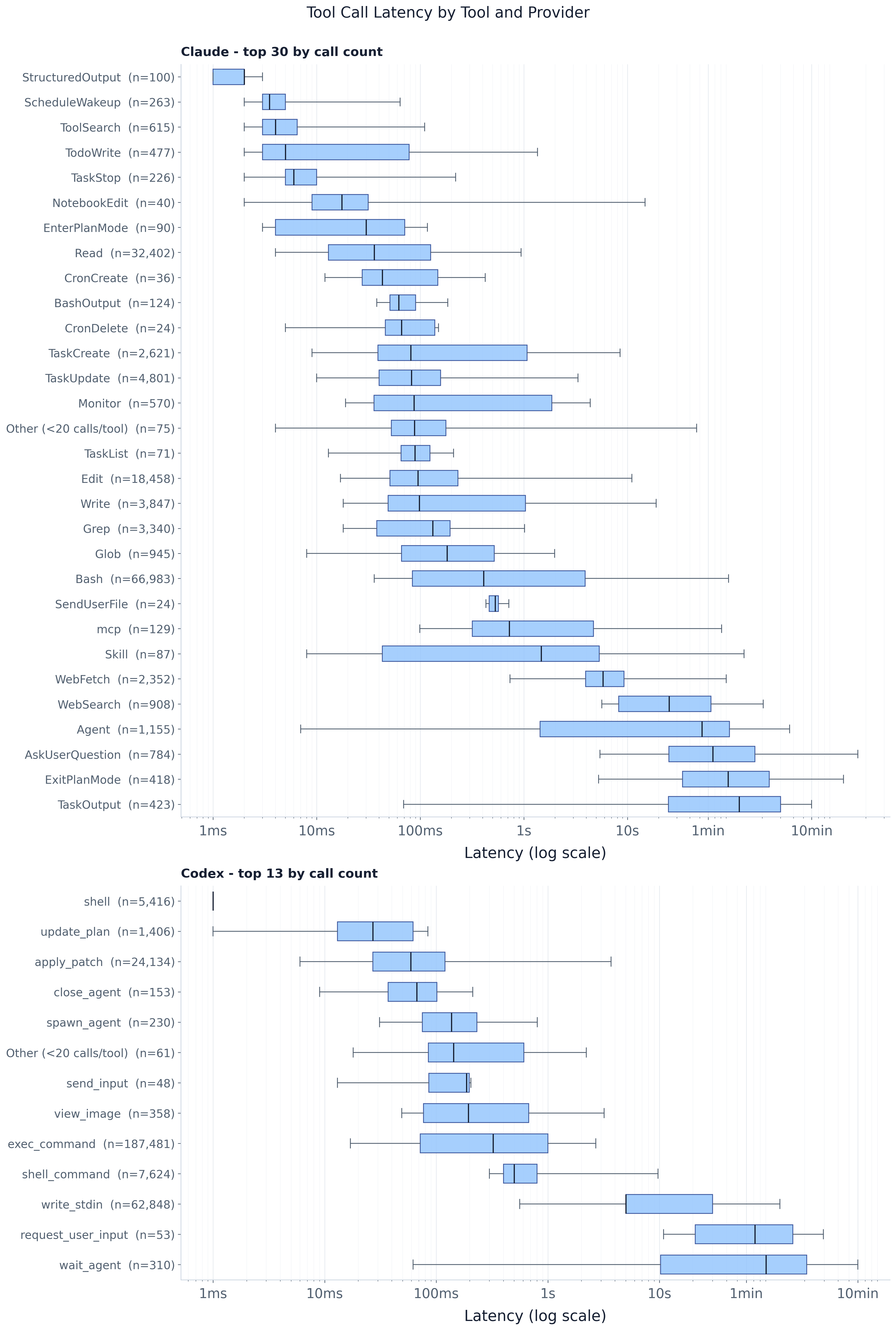
profiles that per-call latency four ways: a per-tool/per-provider box-and-whisker view, a 
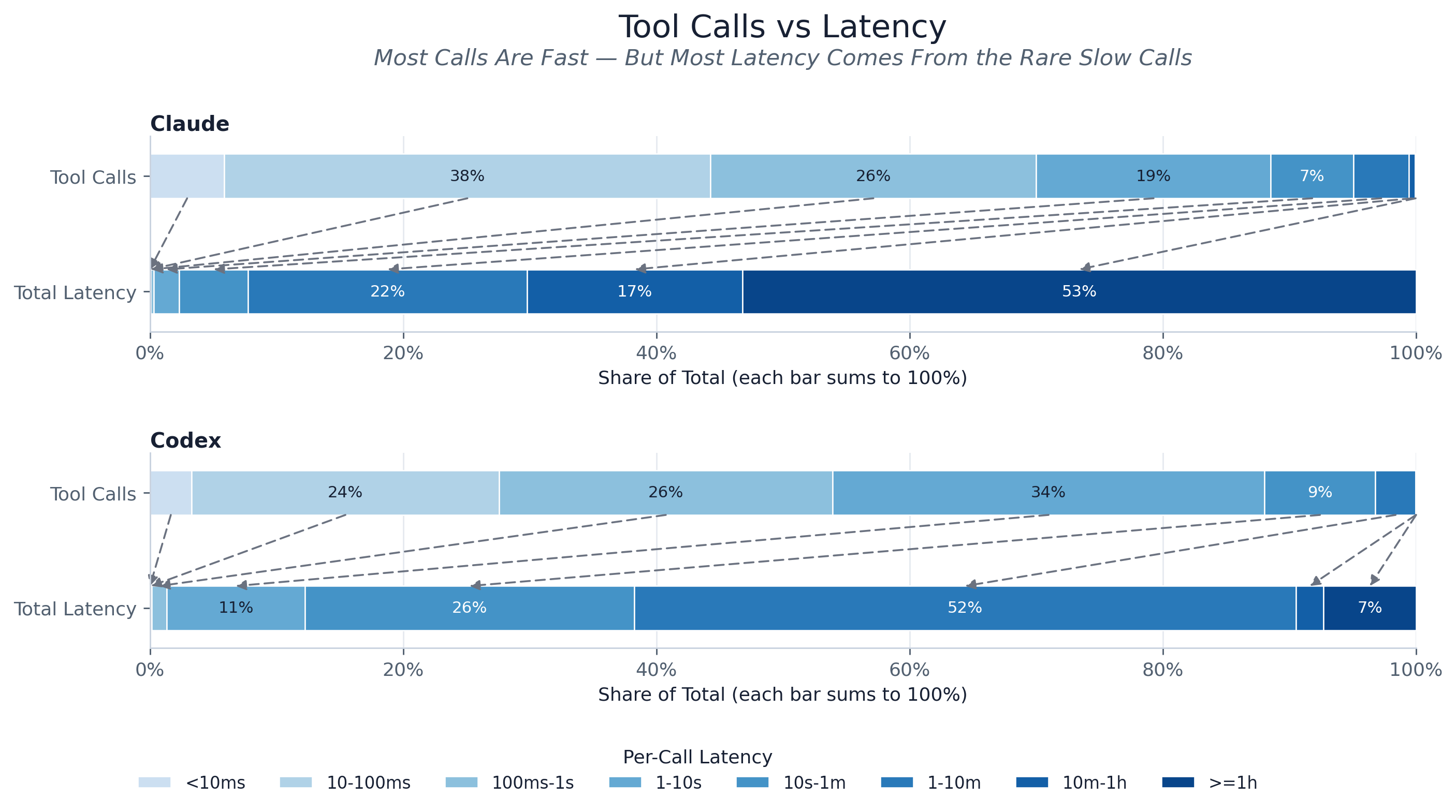
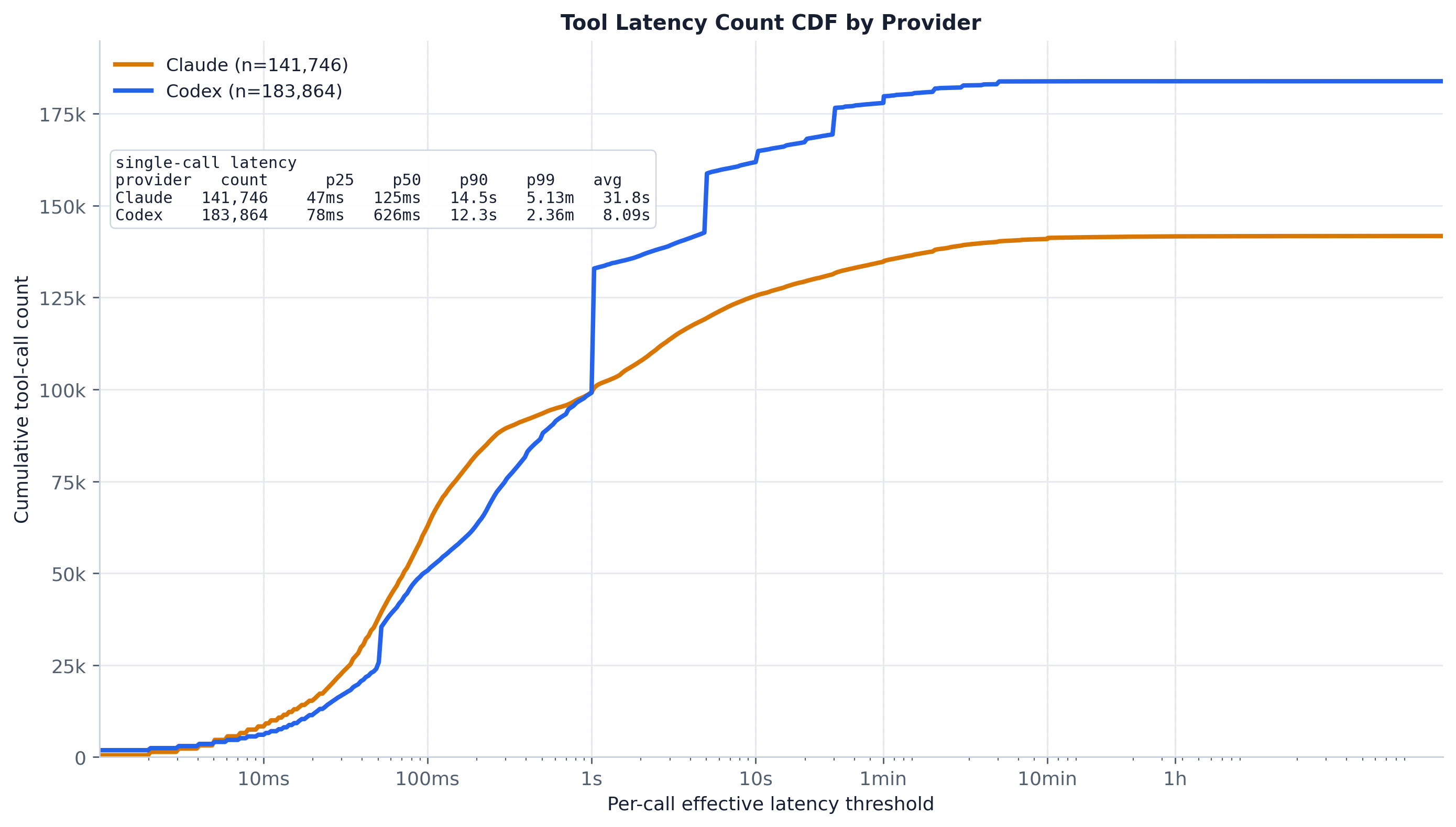
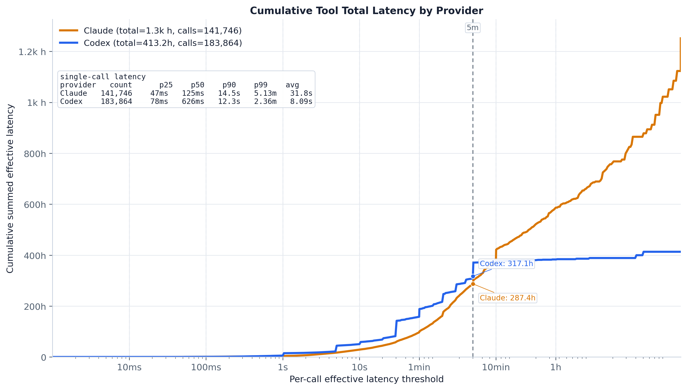
count-vs-latency mass breakdown over coarse latency bins, and two cumulative CDFs (by call count and by summed latency) over the per-call latency threshold.

Method and assumptions:

  • Effective tool latency = tool_internal_latency_ms if present, else tool_wall_latency_ms (= result_at − emitted_at; the shared trace_db.EFFECTIVE_TOOL_LATENCY_MS_SQL precedence — the legacy latency_ms field is not in the normalized data). Internal timing is the runner-reported duration (Codex wrapper Wall time, Claude durationMs).
  • Only strictly-positive latencies feed the distribution. A call with no effective latency is counted as missing_latency; a call with a non-positive effective latency is nonpositive_latency — neither enters the boxplots, bins, percentiles, or CDFs (matching the old ToolStats).
  • MCP tools are merged (figure only). Any tool whose name starts with mcp_ is aliased to a single mcp bucket; the long server-qualified names are individually rare. CSV summaries keep the raw, unaliased names.
  • Rare tools collapse (figure only). Tools with fewer than --min-tool-calls-for-plot provider-local calls (default 20) fold into one Other (<N calls/tool) box. CSV summaries keep full per-tool detail.
  • CDFs are additive over calls. Latency totals sum per call — parallel tools are not collapsed into wall-clock time, so the total-latency CDF measures attributed work, not elapsed session time.
  • Exact, not sampled. Box quartiles, whiskers, percentiles and CDFs are computed over every positive effective latency pulled from SQL. The old per-tool 50k reservoir sampler is gone, so the summary CSV reports sampled=False and sample_count = the full latency_count for every tool (previously the two highest-volume tools, exec_command and Bash, were reservoir-sampled).
Figures 4
Per-tool latency distribution.
Fig. 1Per-tool latency distribution.

Per-call latency spans many orders of magnitude and the spread is tool-specific, not provider-wide. Reading the panels (Claude and Codex, top tools by call count, log-scale x):

  • Boxes are the IQR, the inner line the median, whiskers the 5th/95th percentiles; outliers beyond are suppressed (showfliers=False), so the chart reads as the bulk of the distribution.
  • Fast file/edit primitives (Read, Edit, Grep, apply_patch) cluster in the tens-to-hundreds of milliseconds with tight boxes; blocking tools — shell execution, agents, plan/question prompts, wait_agent/request_user_input — sit seconds-to-minutes to the right with much wider boxes.
  • Tools are picked per provider by call count (top --top-tools) then ordered by median latency, so vertical position reads as “typical slowness”; the long server-qualified mcp_* tools are merged into one mcp box and the rare tail into Other.
Tool-call count share versus summed-latency share.
Fig. 2Tool-call count share versus summed-latency share.

The headline asymmetry: most calls are fast, but most time is spent in the rare slow calls. Each provider gets two 100%-stacked bars over the coarse latency bins — tool-call share on top, summed- latency share below — with dashed arrows tying each bin’s slice between the two.

  • For both providers the call-count mass sits in the sub-second bins, while the latency mass shifts hard right into the 1s–1m/1–10m bins (Claude ~53% of latency in 1–10m; Codex ~52% in 1s–1m).
  • This is the classic heavy-tail signature: optimizing the median tool call barely moves total tool time; the long-running outliers dominate the budget.
Latency CDF by provider.
Fig. 3Latency CDF by provider.

Cumulative tool-call count at or below a per-call latency threshold, per provider. The inset table carries exact p25/p50/p90/p99/avg.

  • Codex’s curve rises later but steepens sharply around the ~1s mark (a near-vertical step where a large block of write_stdin/exec_command calls land at similar latencies), then saturates; Claude rises earlier and more smoothly (median ~125 ms vs Codex ~626 ms).
  • Both curves flatten well before the minutes range — the overwhelming majority of calls resolve in under a few seconds, confirming the long tail is a small fraction of calls.
Summed tool-latency CDF by provider.
Fig. 4Summed tool-latency CDF by provider.

The same threshold sweep weighted by summed latency (in hours), i.e. where the aggregate tool time accumulates. The dashed 5m reference marks how many hours come from calls faster than five minutes.

  • Both curves stay near zero until the seconds-to-minutes range, then climb steeply — the bulk of the hundreds of cumulative hours is contributed by calls in (and beyond) the minutes range, even though those calls are rare (per the count CDF).
  • Claude accumulates more total tool-hours overall and keeps climbing into the multi-hour tail; Codex’s total plateaus earlier. Because latency is additive over parallel calls, treat these totals as attributed tool work, not elapsed wall-clock session time.
Reference

Code structure

plot.py is a thin query→shape→plot pipeline over the shared trace DuckDB:

  • _per_tool_query(plot_name_expr, *, by_provider) — the shared per-tool aggregation: normalizes the tool name (blank/NULL → <unknown-tool>), applies the effective-latency precedence, and emits per bucket the call/latency_count/missing_latency/nonpositive_latency/error_calls counts, latency_sum/min/max, the exact list(eff) of positive latencies, and a first-appearance first_seen ordinal. plot_name_expr selects the raw name (CSV) or the mcp_*mcp alias (figure); by_provider splits per rounds.provider.
  • load_tool_stats(con) — global {tool_name: ToolStats} for the summary CSV (raw names, no collapsing), inserted in first-appearance order so the stable sort(key=calls) reproduces the old dict-order tie-break.
  • load_tool_stats_by_provider(con, *, min_calls) — per-provider stats for the boxplot with the MCP merge in SQL, then the rare-tool collapse in Python; real tools are inserted in alphabetical plot-name order (the old merged-dict order) with Other appended last, pinning equal-call ties.
  • load_tool_latency_values_by_provider(con){provider: [positive latency, …]} feeding both CDFs (exact, no reservoir).
  • load_tool_latency_bins(con, *, by_provider) — the 8 coarse TOOL_LATENCY_BINS_MS half-open bins (call/error counts + summed latency), global and per-provider.
  • plot_* / write_* — the four figures and four CSVs.
  • main() — wires the standard trace_db CLI (--db | -i/--input | -o/--output-dir) and embeds the self-contained PNG sidecar.

The matplotlib 3.9 labelstick_labels boxplot-kwarg rename is handled by the _BOXPLOT_LABEL_KW shim so the figure also renders under the matplotlib 3.8.x bundled with Pyodide (the web Analyze tab). The data layer (parsing, surrogate keys, schema) lives in artifacts/utils/trace_db.py; see artifacts/utils/DB_SCHEMA.md.

Running it

# default merged trace, output next to this README
uv run python artifacts/tool_calls/tool_latency_distribution/plot.py

# a specific trace (materialized to a temp DuckDB cache on first use)
uv run python artifacts/tool_calls/tool_latency_distribution/plot.py -i trace/sample.jsonl

# a prebuilt DB (run_all.py's build-db step passes this), into a chosen dir
uv run python artifacts/tool_calls/tool_latency_distribution/plot.py --db /tmp/trace.duckdb -o /tmp/out

Useful flags: --top-tools (max boxes per panel, default 30), --min-tool-calls-for-plot (rare-tool collapse threshold, default 20).

Outputs

Written to -o (default this folder):

  • tool_latency_by_tool.png — per-provider box/whisker panels of per-call latency by tool.
  • tool_latency_summary.csv — full per-tool stats (raw names): calls, latency_count, missing_latency, nonpositive_latency, error_calls, mean_ms, min_ms, p50/p90/p99_ms, max_ms, sample_count, sampled, providers.
  • tool_latency_weighted_bins.png / .csv — tool-call count vs summed-latency share over the 8 coarse latency bins.
  • tool_latency_count_cdf_by_provider.png / .csv — cumulative tool-call count ≤ a latency threshold, per provider.
  • tool_total_latency_cdf_by_provider.png / .csv — cumulative summed latency from calls ≤ a threshold, per provider.

Each PNG is self-contained — it embeds this README, the CSVs, and the plotting code. Unpack with python artifacts/utils/png_sidecar.py extract <png>.

SyFI Trace Atlas · experiment detail