
For each agent step, how large is the input prompt and how is it split between the cached prefix it reuses and the newly appended tokens it must pay for?
For each agent step, how large is the input prompt and how is it split between the cached prefix it reuses and the newly appended tokens it must pay for?
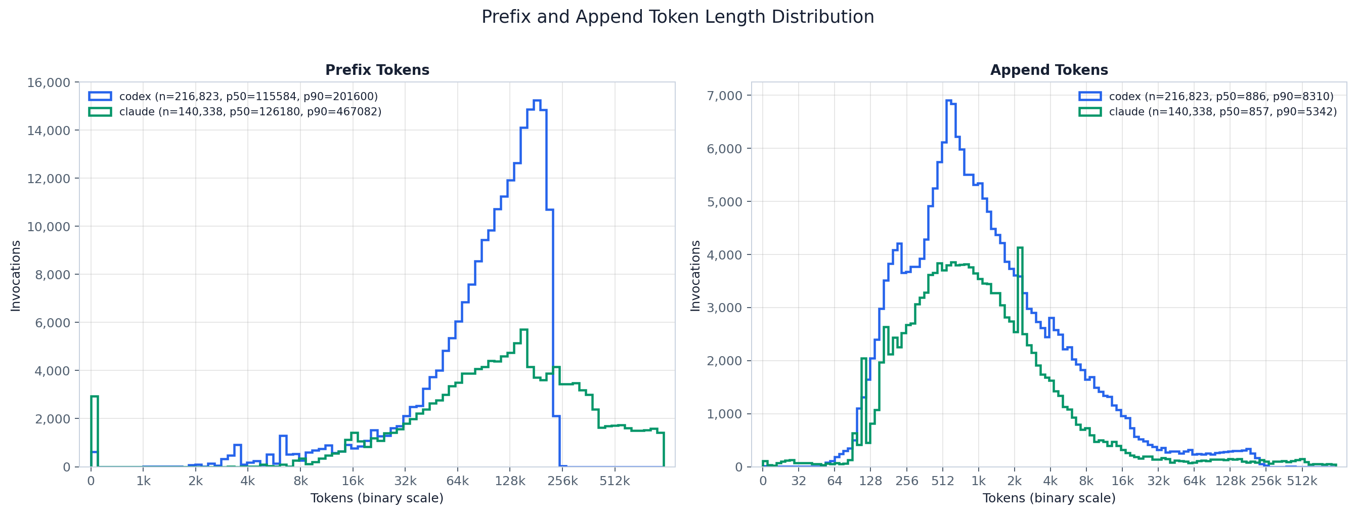
The two histograms sit roughly two orders of magnitude apart. The prefix (cached) curve
piles up far to the right — a median step replays about 141k cached tokens for Claude and 120k for
Codex — while the append curve is centered down near one thousand tokens (median 992 tokens for
Claude, 1,086 for Codex), the only slice a step is freshly charged for. The legend’s p50/p90
quantify the gap, exact over all steps. The takeaway is the central fact of a coding agent’s input:
each step overwhelmingly replays accumulated context and pays for only a thin new margin on top.
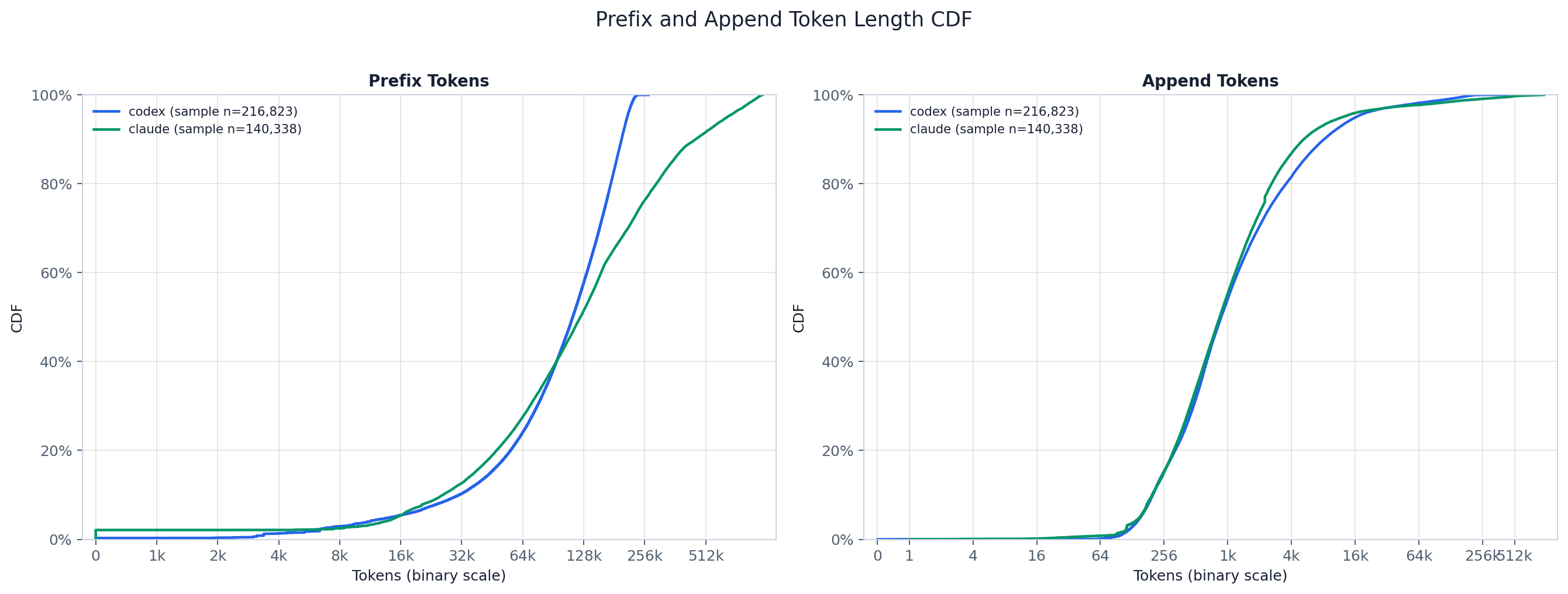
The CDFs make the separation explicit. The prefix curve rises late and keeps climbing into the hundreds-of-thousands range — Claude’s longer context window stretches its prefix tail to a p99 near 920k tokens, while Codex saturates closer to 238k — whereas the append curve saturates early because most appends are tiny. Read where each curve crosses 50%/90% to compare a provider’s typical input cost against its tail, and note that the two providers diverge mainly in the prefix tail, not the append body.
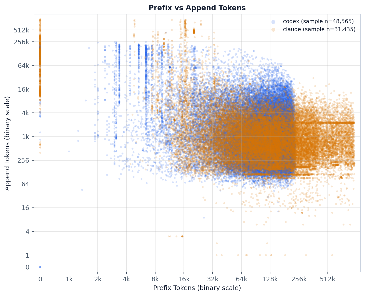
The scatter exposes the joint structure behind the two marginals (this is the paper’s
fig:prefill_append_relationship). Most steps cluster at a prefix of 32k–128k with an append of
256–8k, but two regimes separate out. A small-prefix group (below ~16k) carries comparatively
large appends — these are prefix-cache misses and cold initial prefills, where little is cached
so most of the prompt is paid for as new. The large-prefix group appends little — ordinary
in-session growth, where a step stacks just one tool result or user turn onto an already-cached
context. So a large reused prefix does not imply a large append; the two effectively trade off.
This is a deterministic visual subsample (up to --pair-sample-size points), so read it for shape,
not exact density — use the CSV/CDF for quantitative reads.
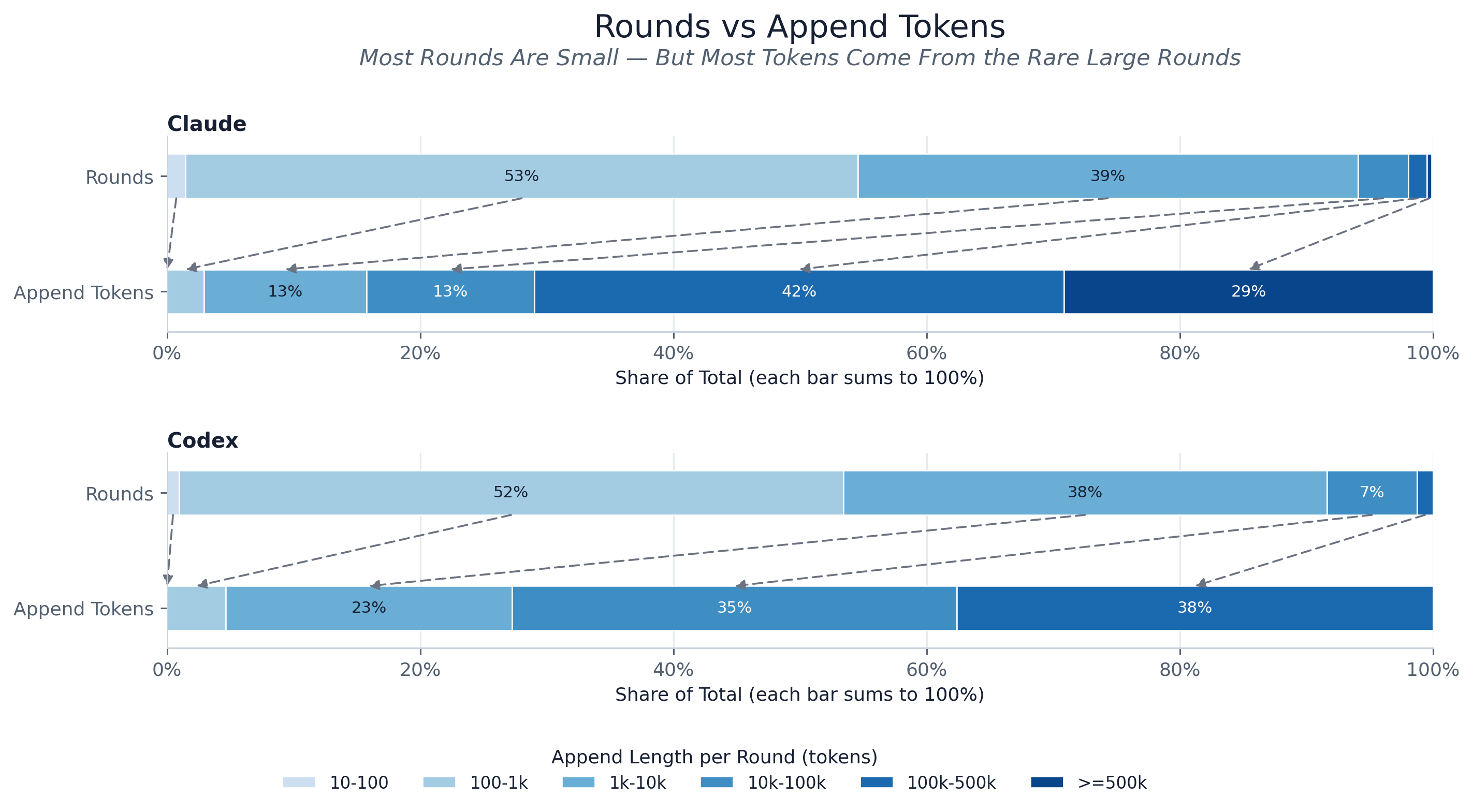
Two stacked bars per provider — step share on top, append-token-mass share below — over the same
append-length buckets (the paper’s fig:prefill_weighted_bar). The two bars invert each other: over
90% of steps append fewer than 1k tokens, yet more than 70% of all appended tokens come from
the rare steps that append 10k or more. The arrows from the count bar down to the mass bar make the
point — even though almost every step is tiny by count, the prefill workload is dominated by a
small tail of large-append steps. That tail is where new-token spend, and the cost of cache misses,
actually concentrates.
Every agent step in the trace carries an input-token accounting:
input_tokens_total = prefix_tokens + newly_append_tokens.
cache_read_input_tokens; Codex cached_input_tokens).input_tokens + cache_creation_input_tokens; Codex input_tokens_total − cached_input_tokens).
See ../../../docs/prompt_cache_accounting.md for the full cache-accounting derivation.This experiment renders the prefix/append distributions (histogram + CDF), a prefix-vs-append scatter, and a token-mass-weighted view of append lengths.
Method and assumptions:
sampled column is
always False and sample_count equals the full count.) Percentiles use np.percentile
(linear interpolation); the mean reproduces the old running float sum exactly by summing the
per-group values in ingest (round_pk) order.>= 0 (the old NumericTracker’s
allow_zero rule); nulls feed missing, negatives feed invalid. The append-weighted bins and
the scatter use rows where both prefix and append are >= 0 (the old loader’s pair gate).--group-by (default provider; also model / provider_model), with
<unknown-provider> / <unknown-model> COALESCE fallbacks mirroring the old group_key.--pair-sample-size, default 80k). Instead of
the old reservoir, the subsample is chosen in SQL by a Knuth-multiplicative hash of the surrogate
key: ORDER BY (round_pk * 2654435761) % 1000000, round_pk LIMIT <pair-sample-size> over rows
with prefix_tokens >= 0 AND newly_append_tokens >= 0. This is reproducible across DB builds and
engines but is not the old reservoir, so the scatter figure is not byte-compatible with the
pre-migration run (the CSVs are).plot.py is a query→shape→plot pipeline over the shared trace DuckDB:
load_token_groups(con, *, group_by) — per-group prefix/append MetricStats (every valid value
in ingest order, plus missing/invalid counts) and the group’s total rows, plus an all
group. MetricStats.summary() derives count/mean/min/max/percentiles exactly.scatter_pairs(con, *, group_by, sample_size) — the deterministic (group, prefix, append)
visual subsample described above.append_bins(con, *, by_provider) — the global and per-provider append-token weighted bins
(steps + summed append tokens per half-open bucket), exact over the pair-gated rows.plot_token_histograms / plot_token_cdfs / plot_prefix_append_scatter /
plot_append_weighted_bins — the figures (matplotlib behavior unchanged from the pre-migration
script).write_token_summary / write_append_weighted_bins — the two CSVs.main() — wires the standard trace_db CLI (--db | -i/--input | -o/--output-dir) and
embeds the self-contained PNG sidecar.The data layer (parsing, surrogate keys, schema) lives in artifacts/utils/trace_db.py; see
artifacts/utils/DB_SCHEMA.md.
# default merged trace, output next to this README
uv run python artifacts/llm_generation/prefix_append_distribution/plot.py

# a specific trace (materialized to a temp DuckDB cache on first use)
uv run python artifacts/llm_generation/prefix_append_distribution/plot.py -i trace/sample.jsonl

# a prebuilt DB (run_all.py's build-db step passes this), into a chosen dir
uv run python artifacts/llm_generation/prefix_append_distribution/plot.py --db "$TMPDIR/trace.duckdb" -o "$TMPDIR/out"
Useful flags: --group-by (provider / model / provider_model), --max-groups (max plotted
groups, default 8), --pair-sample-size (scatter subsample, default 80000).
prefix_append_distribution.png — prefix vs append token histograms.prefix_append_cdf.png — CDFs of prefix / append token length.prefix_vs_append_sample.png — prefix-vs-append scatter (deterministic visual subsample).append_tokens_weighted_bins.png / .csv — token-mass-weighted append bins.token_length_summary.csv — per-group prefix/append quantiles, mean, min/max, and counts.The PNGs are self-contained — they embed this README, the CSVs, and the plotting code
(plot.py + shared artifacts/utils/ modules). Unpack with
uv run python artifacts/utils/png_sidecar.py extract <png>.