SyFI Trace Atlas
Trace assistant
Reading the public SYFI pool
357,161 agent steps across Claude & Codex — public, shareable.
Answers run real DuckDB/Python in a sandbox · code is shown
All figures
Session
one continuous trace of work, often spanning multiple requests or problems.
Request
one user input through the agent's final response.
Agent step
one model call inside a request.
User-initiated step
an agent step started by user input.
Tool-triggered step
an agent step started by a tool result.
Overview

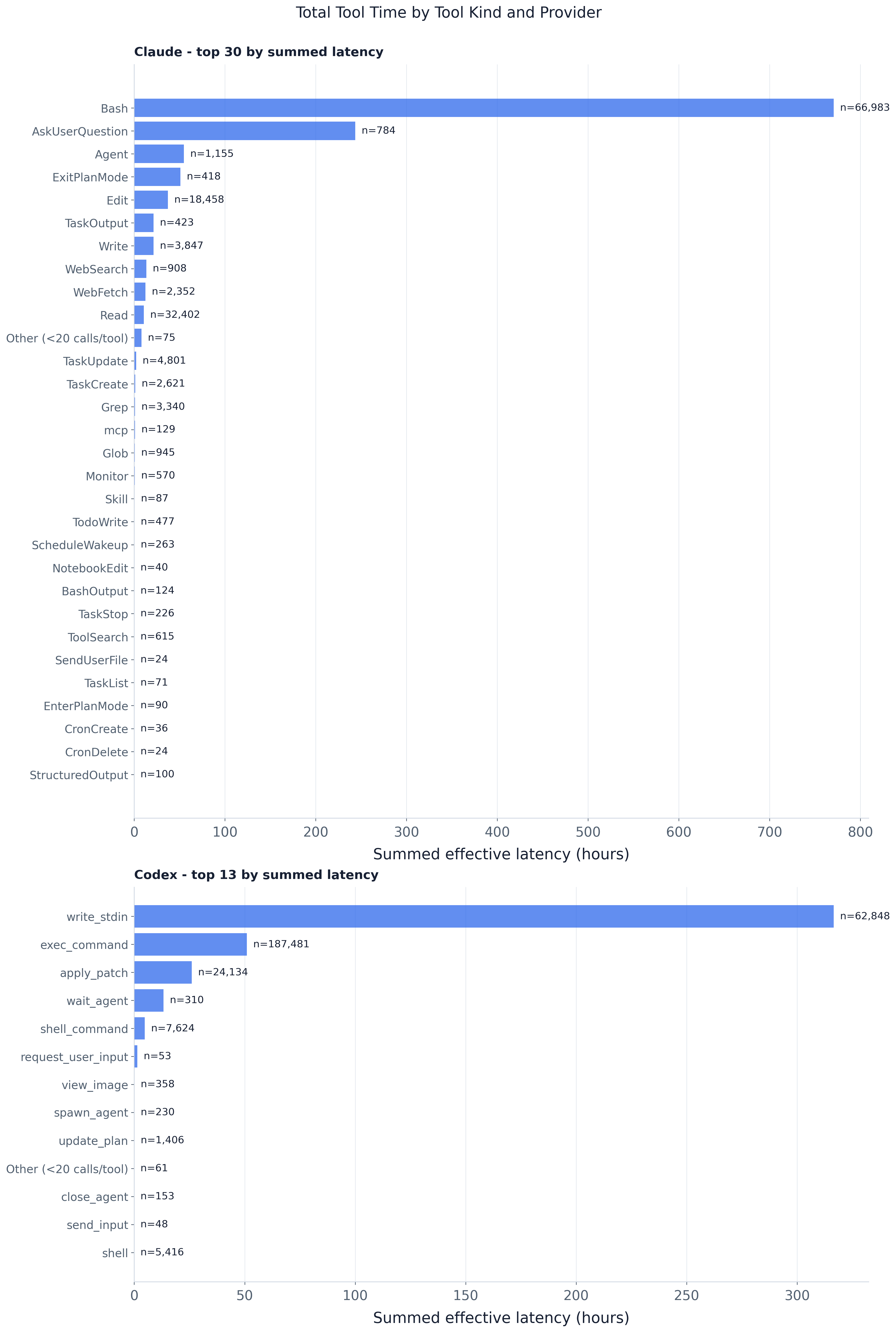
Across all tool calls, which tool kinds account for the most total effective time — separately for Claude Code and Codex?

Every agent step in the trace carries a tools[] list of tool calls, each with a measured latency. This experiment attributes that latency to tool kinds and asks where the aggregate tool-execution time goes, rendering one horizontal-bar panel per provider with tools ordered by summed latency (each bar annotated with its call count n).

Method and assumptions:

  • Effective tool latency = tool_internal_latency_ms if present, else tool_wall_latency_ms (the shared trace_db.EFFECTIVE_TOOL_LATENCY_MS_SQL precedence; the legacy latency_ms field is not in the normalized data). Only strictly positive latencies contribute to a tool’s summed/averaged time; calls with no effective latency are counted as missing_latency_calls.
  • Additive over calls. Latency is summed per tool kind. Parallel tool calls are not merged into elapsed wall-clock time, so this measures attributed work, not end-to-end session time.
  • One row per call. We aggregate entries in tool_calls (the UNNESTed tools[]), not agent steps.
  • MCP tools are merged (figure only). Any tool whose name starts with mcp_ is aliased to a single mcp bucket; the long server-qualified names are individually rare. The CSV keeps the raw unaliased names.
  • Rare tools collapse (figure only). Tools with fewer than --min-tool-calls-for-plot provider-local calls (default 20) are summed into one Other (<N calls/tool) bar. The CSV keeps full per-tool detail — nothing is dropped from the data, only from the plot.
  • Exact, not sampled. Sums, counts and averages are computed over all tool calls in SQL (the old per-tool reservoir sampler is gone), so the totals are exact.
Figures
Total effective tool time by kind and provider.
Fig. 1Total effective tool time by kind and provider.

Tool-execution time is dominated by a handful of long-running tool kinds rather than spread evenly across the tool vocabulary. Reading the panels:

  • The ranking is by summed latency, so a tool can top the chart either by being called very often (high n) or by being individually slow (high avg_latency_ms in the CSV) — the n= annotation separates those two regimes at a glance.
  • Shell/agent and plan/question tools (which block on real work or on the user) carry far more aggregate time than fast file primitives, even when the latter are called more frequently.
  • Because latency is additive over parallel calls, these totals are attributed work, not wall-clock session time; treat them as “where tool effort accumulates,” not elapsed duration.
  • The per-tool CSV (latency_share, avg_latency_ms, missing_latency_calls) gives the exact figures behind each bar, including the long tail collapsed into Other in the plot.
Reference

Code structure

plot.py is a thin query→shape→plot pipeline over the shared trace DuckDB:

  • _tool_time_query(plot_name_expr, *, by_provider) — the shared aggregation: normalizes the tool name (blank/NULL → <unknown-tool>), applies the effective-latency precedence, and emits per-bucket calls, latency_count, missing_latency, error_calls, latency_sum, plus a first-appearance first_seen ordinal for a deterministic tie-break. plot_name_expr selects the raw name (CSV) or the mcp_*mcp alias (figure); by_provider adds the rounds.provider join.
  • load_tool_time(con) — global {tool_name: ToolTimeStats} for the CSV (raw names, no collapsing).
  • load_tool_time_by_provider(con, *, min_calls) — per-provider stats with the MCP merge done in SQL and the rare-tool collapse in Python (summing is order-independent).
  • plot_tool_total_time_by_kind(...) — the per-provider summed-latency panels.
  • write_tool_total_time_by_kind(...) — the full-detail CSV.
  • main() — wires the standard trace_db CLI (--db | -i/--input | -o/--output-dir) to the above and embeds the self-contained PNG sidecar.

ToolTimeStats ties are broken by first_seen (min global call ordinal) so output is stable across DB builds — GROUP BY order is not. The data layer (parsing, surrogate keys, schema) lives in artifacts/utils/trace_db.py; see artifacts/utils/DB_SCHEMA.md.

Running it

# default merged trace, output next to this README
uv run python artifacts/tool_calls/tool_time_by_kind/plot.py

# a specific trace (materialized to a temp DuckDB cache on first use)
uv run python artifacts/tool_calls/tool_time_by_kind/plot.py -i trace/sample.jsonl

# a prebuilt DB (run_all.py's build-db step passes this), into a chosen dir
uv run python artifacts/tool_calls/tool_time_by_kind/plot.py --db /tmp/trace.duckdb -o /tmp/out

Useful flags: --top-tools (max bars per panel, default 30), --min-tool-calls-for-plot (rare-tool collapse threshold, default 20).

Outputs

Written to -o (default this folder):

  • tool_total_time_by_kind.png — provider-paneled total effective time per tool kind.
  • tool_total_time_by_kind.csv — full per-tool totals: tool_calls, valid_latency_calls, missing_latency_calls, error_calls, total_latency_ms/_s/_hours, latency_share, avg_latency_ms.

The PNG is self-contained — it embeds this README, the CSV, and the plotting code. Unpack with python artifacts/utils/png_sidecar.py extract <png>.

SyFI Trace Atlas · experiment detail